
Before accomplishing simulation for the entire aircraft, I tried draft simulation the entire rotor on a ready to use framework for the CFD simulation, in particular, it was FreeFEM++ framework. The demand was to obtain entire picture of interference the wings for rotated rotor in different modes of its operation. I understood that such a task cannot be accomplished for case of viscid flow since only modeling one wing with the viscid flow is a tedious task. Therefore, I limited this task only for inviscid flow in two-dimensional space. Below are some details and results of this, which can be useful for anyone for such a drafting.
Let begin with explanation of the inviscid flow simulation concept. The inviscid flow means that there missed any losses related to the flow medium friction. In practice, there are such losses but only in limited spatial domains. Main spatial domain for them is the boundary layer between a surface and the medium, where speed changes from zero to the free speed of the flow. The boundary layer can be with laminar or turbulent flow. The main effect of the laminar flow on a wing flow is its continuation after the trailing edge (TE), like the wing is some longer. But the longer extent is not subject for acquiring forces since it is not a part of wing, which is equivalent for having some drag. The main effect of the turbulent flow, in additional to the effect of laminar flow, is bearing additional kinetic energy of the micro-vortices that it contains, which is subject for dissipating in the after wing’s wake. Therefore, the wing’s wake is another spatial domain for the viscid flow. Finally, there indeed remains a much amount of space between wings that is purely inviscid. For such inviscid flow, energy conservation law acts in the form of the Bernoulli equation that states that sum of the kinetic energy of flow and potential energy pressure is equal to some constant:
ρV2/2 + p = const (1)
Any such flow can be considered as a set of some streamlines, along each of such the Bernoulli equation acts. And the mentioned constant can be same or can be differed between separated streamlines. Therefore, some number can be associated for each streamline, which guaranteed that the constant will be kept. The streamline with the number acts like an equipotential surface in electrostatics, which keep energy of a charged particle unchanged. The electrostatic potential φ there acts as a pure scalar and it is related to the electrostatic field vector E by the equation:
E = -grad φ (2)
This scalar potential is related to phenomena of changing energy of a charged particle when it moves along the vector E, which is opposite to the phenomena of keeping the energy of a small stream volume upon moving along the streamline. However, there is another analogy for a field, which does not require the changing energy of a charged particle moved along it. It is magnetic field, which vector B the potential theory considers as some curl of another vector A that is named as vector-potential:
B = curl A (3)
Considering a speed vector u instead of the vector B, there can be considered some vector-potential for the field of speeds, however direction of such vector-potential should be clarified. The particular case of the interest is 2-D flow in the XY-plane. Therefore, z-component of the vector u is just zero. The curl at the equation (3) requires for such case to have zero-values of the particular derivatives of x and y components in the XY-plane for the vector-potential. Therefore, in view that a potential is defined up to a constant in its exactness, both its x and y components will be zero. Thus, the vector-potential will consist just from one z-component and can be represented by a scalar value ψ:
u = curl ψz (4)
And the components of the vector u will be:
ux = dψ/dy (5a)
uy = -dψ/dx (5b)
In the boundary layer for a viscid flow, a condition exists for non-zero value of the curl of u- vector since the speed gradient there corresponds to a rotation of a stream’s front that is perpendicular to the streamlines. But outside of the boundary layer or just for an inviscid flow, the curl will be zero:
curl u = 0 (6)
A substituting the (4) to (6) will utilize curl of curl identity that by using the operator ∇ is:
∇ ✕ ∇ ✕ ψz = ∇ (∇∙ ψz ) - ∇2 ψz = 0 (7a)
i.e.
curl curl ψz = grad div ψz - ∆ ψz = 0 (7b)
, where the ∆ is the Laplace operator.
The divergence of ψz is equal to zero since the ψ isn’t changing along the Z-axis. Therefore, the equation (7b) will be resulted just to:
∆ ψz = 0 (8a)
or just:
∆ ψ = 0 (8b)
The equation (8b) is the case of potential flow for irrotational stream and it is known as Laplace equation. Additionally, it should be point out that air can be considered as an incompressible liquid when its speed is far from the speed of sound. Mathematically it requires the div u to be equal to zero. The equation (8b) implies this feature indirectly through using the relation (4). Thus, the div u will be zero since the divergence of any curl is always zero.
Implementation of such Laplace equation for modeling free airflow, i.e. pure ambient case, in the FreeFEM++ framework is a very simple task that requires just addition to the formulation of the equation (8b) a boundary condition for the outer boundary that represents infinity of the airstream. The condition will be just direction of the airstream relative the X-axis under some angle α. For the case when the angle is just zero, entire distribution of the ψ field will be just a ramp in the Y-direction with constant values in the X-direction and with zero value in middle, i.e. :
ψ-infinity = y (9a)
In other case it will be:
ψ-infinity = y∙cos α - x∙sin α (9b)
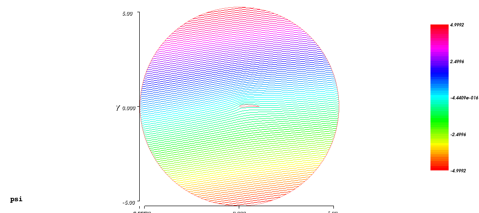
There x and y are just x and y coordinates of any node of any finite element demanded through inclusion in respective border elements under execution of the calculation and represented in the internal variables of the framework under the same names. Below is a result of such environment modeling for the case when the α equal to 8°:
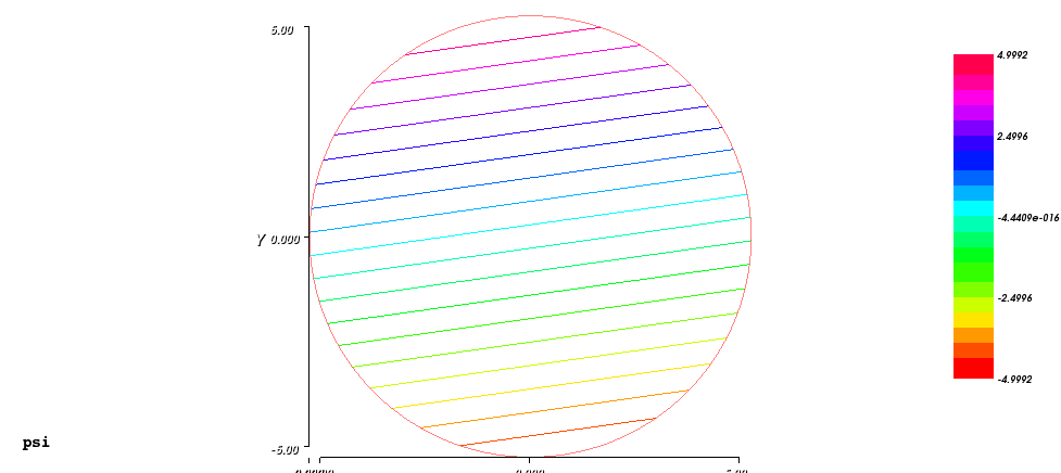
The infinity border here is a circle with radius of 5 units and the ψ varies between -5 and 5.
The field of the speeds u was derived from the ψ distribution using the equations (5a) and (5b). Magnitudes of it are represented below:
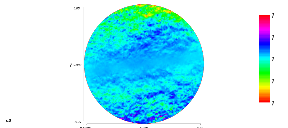
The image pictures noises of the speed around the unity value. The field of the pressure coefficients was derived from the square of the magnitude of the speed field utilizing the equation (1) considering the ρ/2 equal to unity, as well as the “const”:
Cp = 1 - u02 (10)
Thus, the “const” values for all streamlines are the same, which is a specific feature for the irrotational potential flow. And the 1 in the equation (10) represents the quad of the speed for any streamline at infinity.
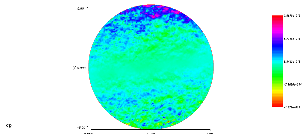
The image above pictures noises of the pressure coefficients around the zero values. The noises are very low, around 10-13 and the entire image is complimentary to the previous. So, noises on the previous image are also of a very low magnitude order.
Now, let consider how the ambient case should be changed in order to model the rotating rotor in the center. The potential flow method is strong in its simplicity by not requiring exercising the time domain. On other hand, the rotor is moving over time and has some phase state at each moment, which hints toward using the time domain. This at first look contradictory relation can be resolved by considering the rotor is steady and is snapshotted in its particular phase and the air is in the superposition of the background stream flow with the air rotating in the direction that opposite to the direction of the actually rotating rotor. Thus finally, there requires a formulation for potential flow that should provide the result that is the required kinematic superposition of the background stream and the rotating stream. Having such rotating stream will break the equation (6) by a non-zero curl, which consequently breaks the equation (8b) requiring now at the right hand side some function related to the non-zero curl distribution:
∆ ψ = f(x,y) (11)
The last equation is known under name of Poisson equation. Actually, the distribution of speed of rotation looks as a cone centered in the origin, where the speed is zero. The curl of such speed distribution will be flat distributed with a constant value equal to du0/dr, where the r is just a radius from the origin. However, such constant value is not sufficient to provide the formulation with the required effect due to the special case in the origin, where the speed equal to zero. Thus, the function f(x,y) should behave like a value that is near to some constant except for the vicinity of the origin. From the point of view of the said cone, this could be understood also like the cone will be substituted by a rotating hyperbola appeared from a big distance like the said cone. I found such a function experimentally. At first, I considered some kernel function f00, which is just a rotating parabola:
f00 = x2 + y2 (12)
At second, I considered some function f0, which is the kernel function scaled on a coefficient Ku in order to reflect the actual speed of rotation:
f0 = Kuf00 (13)
The Ku coefficient I defined as:
Ku = 0.5Umax/Rmax (14)
, where: Rmax is generally a known radius and particularly just the maximal radius of the considered space; Umax is generally a known linear speed of rotation for the known radius and particularly just the speed adjusted to the Rmax becoming the maximal speed of rotation for the case. The coefficient 0.5 in the definition (14) compensates for the coefficient 2 arising upon getting derivatives from the function f00.
The function f0 should be added to the boundary condition (9b) for the airstream infinity as:
ψ-infinity = y∙cos α - x∙sin α + f0 (15)
The function f utilizes the kernel function f00 and the Ku coefficient appearing as:
f = 3.99513Kuf000.001 (16a)
, or more exact version:
f = 3.99915Kuf000.0001 (16b)
The the first coefficient value there that is near to 4 is adjusted to the power value used with the f00 function. Below is a result of the environment modeling, using the (16b) version of the function f, for the case when the α equal to 8° and the Umax is just 1:
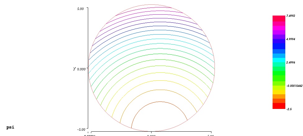
The stream lines there have values those reflect total kinetic energy of air with a minimum value just on the low side of the border, where the background speed should be compensated by the speed of rotation from the point of view of the considered rotor. The field of the speeds u can be calculated by the equations (5a) and (5b), like as for the background case. Magnitudes of it are represented below in the iso-line form:
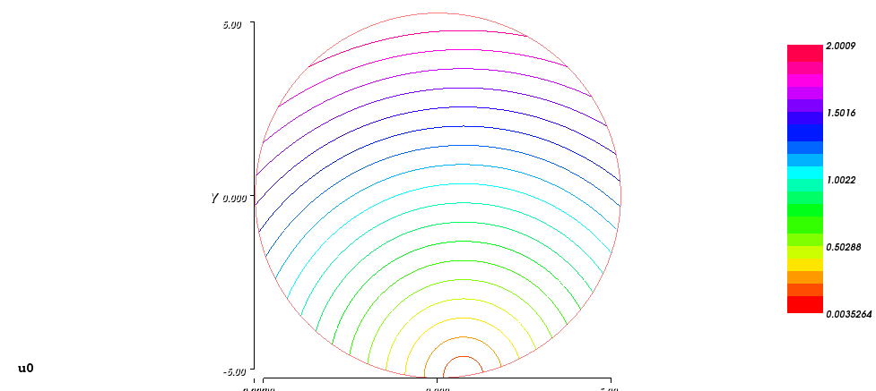
These iso-lines on the picture are equidistant that reflects the perfect cone distribution with a zero-value just on the border. Thus, the total field distribution composed from the background stream and the speed of the rotation also will be a cone-like distribution with its center in the point, where the two kinds of the speeds compensate each other.
The field of the pressure coefficients also can be derived from the equation (1), like the equation (10) for the background case. However, there is a formal difference: the constant values for different stream lines are not same since each one represents air with a different total energy. Nevertheless, this fact can be simply ignored since the pressure coefficients will be used for calculating the lift coefficients of particular wings by calculation respective integral over the closed circuit of the border of a respective airfoil. This closed circuit integration will nullify the constant pressure error value of the leading edge streamline shared by the entire airfoil border. Such case of the cp-distribution I reference as cp0 and it is represented below:
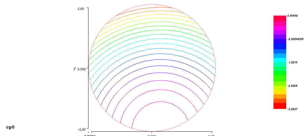
The image above pictures the pressure coefficients associated with the respective streamlines including the said error values since the equation (10) was used for its calculation. The stream line that associated with the speeds compensating point has the unity valued pressure, like for a stagnation point at leading edge of a wing. The stream line associated with the value that equal the background speed of unity has the zero valued pressure. The streamlines associated with highest speeds have negative pressures, like above a wing. Although such cp0 field can be used for calculation the lift coefficients, it cannot be used for investigation the pressures around the airfoils, for which the absolute pressure coefficients are matter. In order to obtain such coefficients, the equation (10) should be modified to the following form:
Cp = U02 - u02 (17)
There U0 is just the value of the speed for a streamline of interest at its infinity or at any other non-disturbed location. For the particular case of the ambient flow that doesn’t have disturbances, the equation (17) will provide a zero valued result. Implementation of this generally means that the streamline associated with the each point of interest should be traced back to such non-disturbed location, for which the speed value U0 should be obtained. A particular implementation can be just finding a correct point at the non-disturbed location, which potential value is the same as the value of the point of interest. For the particular case above, the non-disturbed location is just the circle of the infinity border. Thus, some algorithm can be used, e.g. the step-halving algorithm, for searching a correct position on the circle for the potential known value. Below is the cp-distribution provided by this way for the case above:
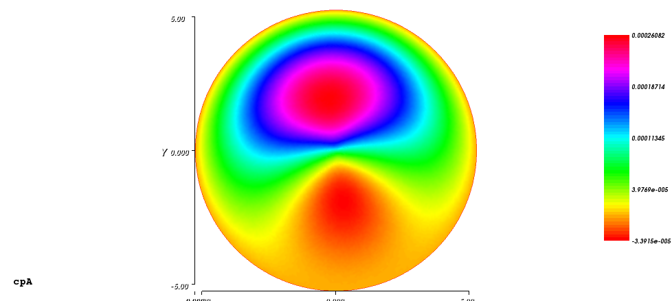
The image above pictures pressure coefficients those are very near to zero. But it is not a noise. It is a systematic errors distribution. For better understand this, the image of streamlines can be over imposed this image. By this way, variations of the pressure can be traced along a streamline. Thus at upper side, a pressure begins with just under zero value, increases with the pace of approaching to the center of the rotating component and continues so in the reverse order. And at the lower side, a pressure begins with zero value, decreases a bit under zero value and so on. Therefore, these systematic errors represent the speeds errors those are maximal at the two central areas. Using the version 16(a) of the function f will provide there a similar result but with errors ten times higher.
Almost the same result image can be produced by a more advanced way than using the time consuming algorithm. The U0 values can be obtained just analytically by using the equation (15) for the boundary condition in order to obtain the x and y values on the circle for the known ψ value. After the values will be obtained from a quadric equation resulted for the equation (15), they can be substituted in a kinematic formulas for the components of the u vector at the circle position. Using the version 16(b) of the function f will provide a result with errors on 15% lower. However, for the 16(a) version, result will be drastically different:
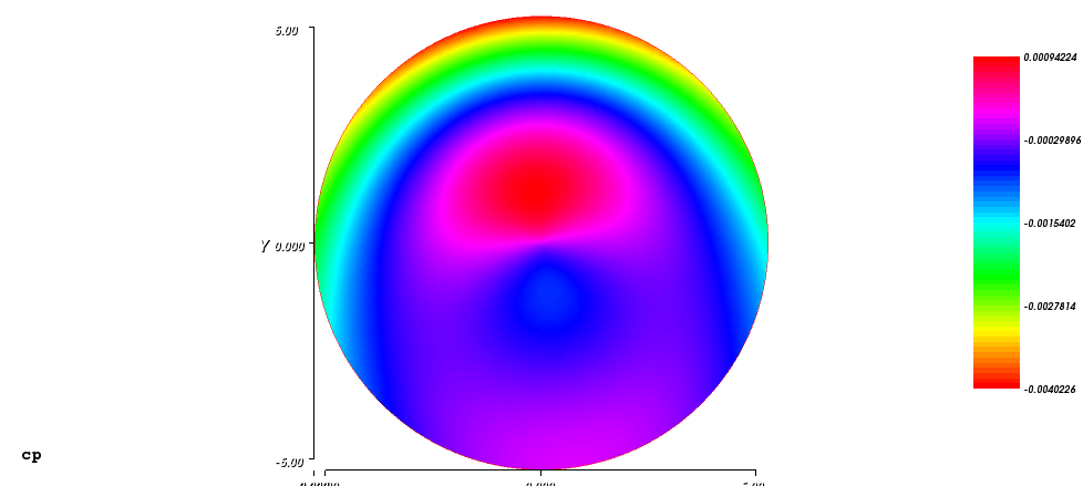
The image above pictures the result, where can see some big and relatively flat area with errors three times less than for the search method. But at upper part, there is a narrow band with errors on 50% higher than for the search method.
Placing a number of airfoils sections in environment of any of explained above ambient flows considers reflecting the case of placing respective number of wings of the respective airfoil geometry without end wing effects with some minimal viscosity. This minimal viscosity is a crucial feature, without which no one wing cannot provide a lifting force. This follows indirectly from the Kutta-Joukowski theorem that requires existence of an air circulation around the wing for the lifting force. The circulation is just the integral along any path around of the wing from the dot product of the path’s tangential vector by the speed vector u. This integral quantity does not depend on the shape of the path and on its distance from the wing, representing by this feature the angular momentum conservation law. Thus, any small volume of air will have its own angular momentum constant upon moving at any position relative the wing. Conservation of this angular momentum requires zero viscosity of the air. However, just having this non-zero circulation can be resulted only if the closed path area has inside it the same amount in the integral of the stream of the curl of the vector u, as the Stokes theorem requires. The last requirement points toward non-zero curl of the vector u contradicting the equation (6) of the inviscid flow condition. For the actual wing, the viscid flow at the particular location of the boundary layer of the wing upon the airstream establishing provides the necessary amount of the curl of the vector u that is referenced under name vorticity and remains kept virtually at the airfoil section area.
At this point, a question arises: how can be the inviscid flow modeling connected with the vorticity feature of the viscid flow? The answer for this will be provided by the history of the aviation theory and practice. The history was resulted in the shapes of particular airfoils. But all of the airfoils have a common feature in the sharp trailing edge, which connection with lifting force of a wing was identified in practice and further explained as having there some vortex under particular circumstances. The vortex is named “starting vortex” or Kutta vortex. And as its name pointing out, the vortex appears only upon start of the wing’s acceleration relative the air. At this point the said vorticity is just singularity at the sharp trailing edge and other segments of the boundary layer are not effective in the same action, generally. The starting vortex provides a source for the effect of having a minimal circulation about the wing, which leads to modifying airflow around the wing. At the time when the circulation still isn’t developed, the near zero balance of it is supported by a bound vortex that virtually placed inside the airfoil section area mainly compensating the starting vortex. This bound vortex reflects a negative circulation of the non-modified airstream calculated over the airfoil section contour, which excludes the starting vortex. Upon modifying the airflow and increasing the overall circulation, the starting vortex is reducing since the modified airflow provides less pressure difference at the trailing edge and less speed difference that powers the starting vortex. The negative bound vortex decreases and changes its sign. Finally, the starting vortex disappears, a stagnation point develops at the trailing edge, the required overall circulation develops fully and the vorticity will be distributed inside of the airfoil section area as the bound vortex indicating that the circulation does not require more power for its developing.
Therefore, from this explanation, a simple condition follows that is known as Kutta condition that in order to retain the stagnation point at the trailing edge for the fine developed airstream, the difference of the pressures or the speeds just above and below the trailing edge should be adjusted near to zero. A condition for implementation of the above condition for the case of the potential flow sounds simpler: the boundary condition for an airfoil should be just a potential value, which effect satisfies the Kutta condition.
Example of implementation the Kutta condition is provided in the tutorial of the FreeFEM++. The example operates directly with potential values without transition to the pressure and speed. For this case, the difference in the potentials is used instead of the pressures difference. More exact, the condition value is: the sum of the differences of the potentials just above and below the trailing edge relative the potential of the wing itself. For the well-adjusted case, this value should be near zero. A number of try and check iterations (actually 3) used for progressively obtaining the correct condition. The value of the condition obtained in a current iteration is used for calculating the wing potential for the next iteration by adjusting the current potential of the wing with inversion of the value from the condition divided on a factor of correction. The factor of correction is just the similar condition value obtained from a special starting calibrating potential flow calculation. This starting calculation uses boundary condition for the infinity of 0 and the boundary condition for the wing of 1.
Below is a result of such potential flow calculation for the airstream with α equal to 8° around the airfoil NACA4410 :
Below is the zoomed view of distribution of the magnitude of the speed u0 around the used airfoil:
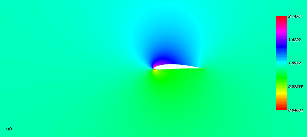
There can see that airflow near the trailing edge is perfectly smooth. Also, there can see the high speed area over the wing and decreased speed area below the wing with the stagnation point some below the leading edge.
Below is the zoomed view of distribution of the pressure coefficients cp around the used airfoil:
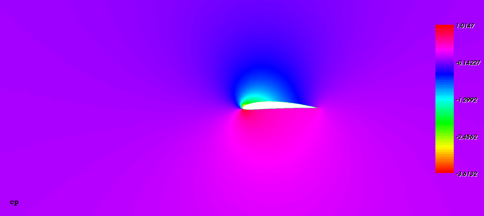
There can see low pressure area above the wing and the high pressure area below the wing.
The final calculation of the potential flow around rotating rotor of the wings was performed with using similar but more elaborated method for adjusting potentials of the wings as for the one steady wing described above. All the potential were modified in parallel, for each of iteration, but the number of such iterations was higher. Below is a result of such potential flow calculation, which utilized the formula 16(a), for the airstream with α equal to 0° around the rotor of ten NACA4410 airfoils rotated with linear winding speed of 30% of the ambient airflow speed and operated in the idealized (just linear transition) alpha mode of the biangular handling with the main alpha angle of 5°, the opposite alpha angle of 2°, the skew angle of 15° and phase of 0°:
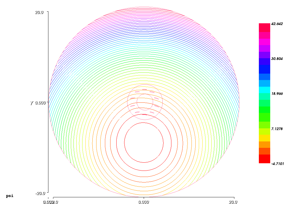
The picture above exposes the radius of infinity of 20 chords of used airfoils, the streamlines with the speeds compensation position that is significantly below the rotor and some very weak deformation of the streamlines below the rotor.
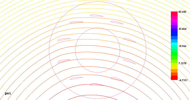
The picture above represents the central zoomed view of the potential distribution of the result. There can see particular interactions of the streamlines with wings.
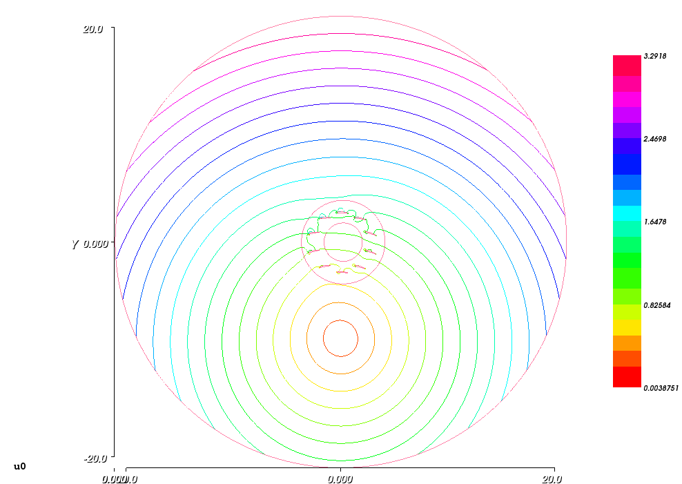
The picture above represents the entire distribution of the magnitude of the speed u0 of the result. There can see that the impact of the wings on the speed disturbing is significantly higher at the upper wings of the rotors, where the local speed of the wings is higher.
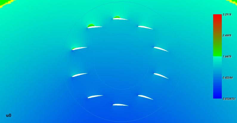
The picture above represents the central zoomed view of the magnitude of the speed distribution u0 of the result. There can see particular speed variations at the wings vicinities, which are more prominent for the upper wings.
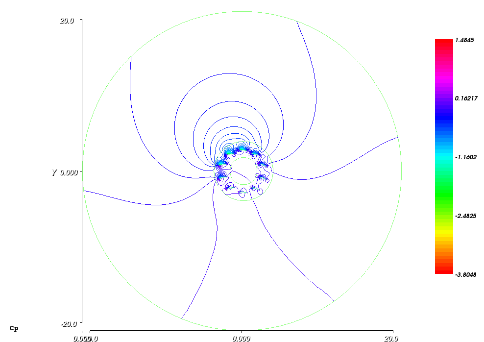
The picture above represents the entire distribution of the pressure coefficients Cp of the result. The Cp calculation used the analytical calculation of the U0 values for the equation (10) on the circular border, where it was possible. But for the remained streamlines that are closed, a pole of the zero speed was found, a connector-line was considered between this pole and the nearest side of the circular border and the U0 values were calculated along the connector from a measured distribution of such values along it. However, such way leads to a shifting the Cp distribution inside the second spatial domain of the closed streamlines on a constant value relative the circular border domain due to using two non-similar kinds of sources of the U0 values. Thus, the shift value was found and used for shifting back the Cp distribution inside the second domain. For instance, the value was just 0.0587. An alternative to this was considered and checked in using the measured values along the circular border instead of the calculated. For this case, the result was directly without the shift but the iso-lines of the Cp were badly conjugated in their directions along the border of the two domains, indicating by this that the first variant is more correct. Therefore, the image above pictures the iso-lines of the Cp perfectly conjugated on the domain border that cannot be saw due to this feature.
Additionally, the picture above exposes a negative pressure envelope developed above the upper wings of the rotor. The envelope was built up due to a cumulative action of the areas of strong negative pressure over the said wings all oriented to the outside.
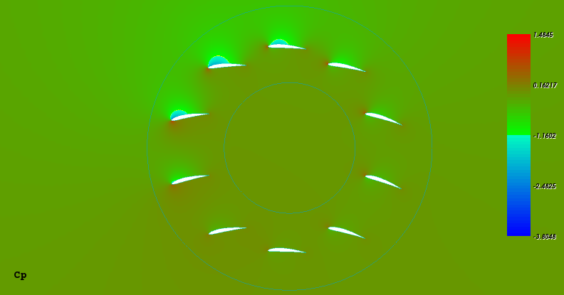
The picture above represents the central zoomed view of the pressure coefficients distribution Cp of the result. There can see particular pressure differences between upper and down sides of the wings, which are significantly more prominent for the four upper-forward wings. Thus, the rotor acts there as a tetra-plane. The maximal Cp value at the legend appears too low for the stagnation point of the center-up wing, to which it is correspond, due to the effect of the negative pressure envelope originated from the wings interference and mentioned above.
The table below provides a result of calculation the wings coefficients using the Cp distribution:
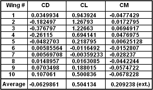
All of the coefficients in the table were calculated for the background airstream. For a single steady wing, the potential flow should provide the drag coefficient CD very near to zero. Thus, the significantly high and negative values of the CD from the table are due to variations of the local streams of respective wings relative the background airstream by the rotation and interference. The moment coefficient for the average result mainly includes an impact from the external moment created by the wings on the rotor’s shaft. Therefore, its value represents the external moment, as well as the consumed power after scaling it on the winding speed.
Below is result of the potential flow calculation for the same rotor parameters, except for the winding speed, which keeps the same value but is for the opposite rotation direction:
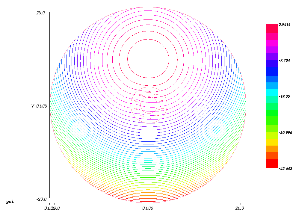
The picture above exposes the streamlines with the speeds compensation position that is significantly above the rotor and some moderate deformations of the streamlines at forward and above the rotor.
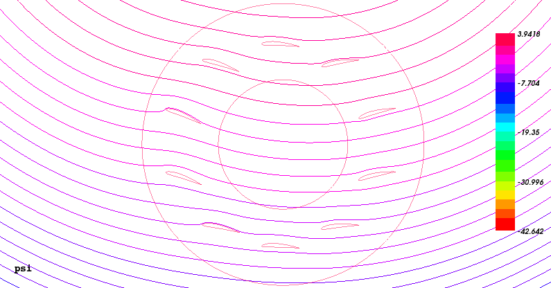
The picture above represents the central zoomed view of the potential distribution of the result. There can see particular interactions of the streamlines with wings, which are more prominent than for the case of the forward rotation.
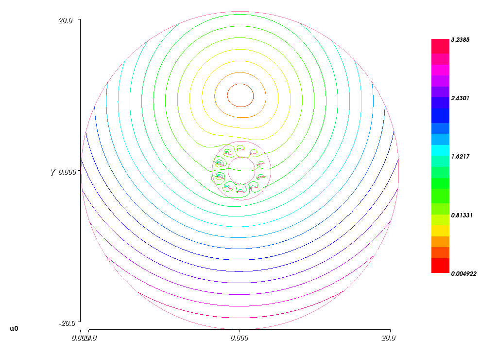
The picture above represents the entire distribution of the magnitude of the speed u0 of the result. There can see that the impact of the wings on the speed disturbing is high not only at the lower wings of the rotors, where the local speed of the wings is higher, but also on the forward-upper wings, which angles of attack is higher than nominal due to the wings interference and the skew value of 15° that is better suits for the opposite rotation.
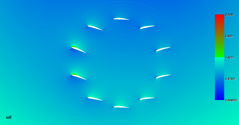
The picture above represents the central zoomed view of the magnitude of the speed distribution u0 of the result. There can see particular speed variations at the wings vicinities, which are more prominent for the forward wings.
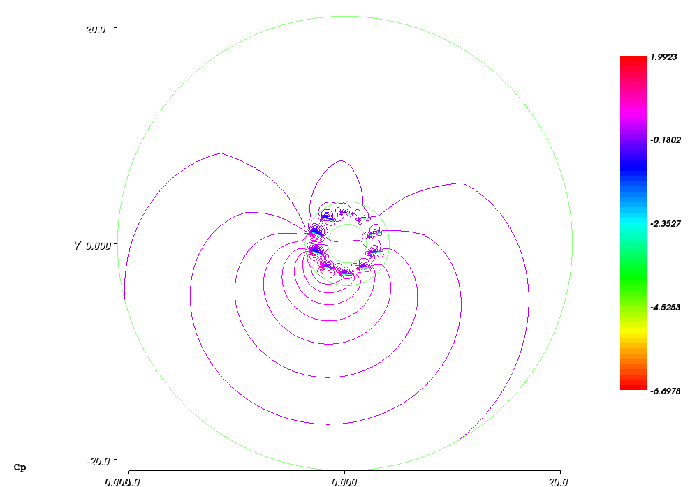
The picture above represents the entire distribution of the pressure coefficients Cp of the result. The iso-lines of the Cp there are not so perfectly conjugated at the closed streamlines domain border as for the previous case of the forward rotation. Nevertheless, it is a best method result since the method of using the measured values on the circular border provides a worsen result.
Additionally, the picture above exposes a positive pressure envelope developed above the lower wings of the rotor. The envelope was built up due to a cumulative action of areas of strong positive pressure below the said wings all oriented to the outside.
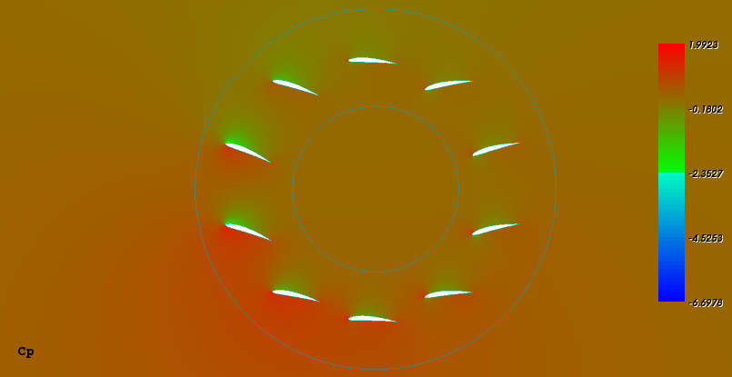
The picture above represents the central zoomed view of the pressure coefficients distribution Cp of the result. There can see particular pressure differences between upper and down sides of the wings, which are significantly more prominent for the four forward-lower wings.
The table below provides a result of calculation the wings coefficients using the Cp distribution:
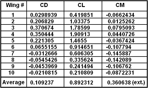
There can see that the lift coefficients are higher than for the case of the forward rotation. This also reflects in the average external moment coefficient pointing out that the rotor provides high recuperative power due to the negative winding speed.
Although the draft simulation method provided the meaningful result, it cannot be used for providing a particular and quantitative result for the liftoplane rotor simulation due to the 2-D limitation and the existence of a feature of incorrect mating the method to the prolate rotor kinematics. This feature is: only the pivots of the wings are in rotation but the wings are rotated back relative the rotor in order to stay near parallel to the stream. This leads to the non-actual airstream flow due to the rotation of the wings in the used draft simulation, especially at the trailing edges, from which the Kutta condition depends that moderates the entire flow. Therefore, after recognizing this drawback, I switched my work toward the simulation method that actually used.
Copyright © 2018-2026 Yuri Feldman - All Rights Reserved